As artificial intelligence models scale from tens of thousands of tokens to massive million-token context windows, standard dense Transformers have collided with an unyielding mathematical barrier: the Quadratic Attention Wall (\(\mathcal{O}(N^2)\)). In standard multi-head attention, computing pairwise token affinity matrices across an 8k sequence requires manageable memory; scaling that sequence to 1,000,000 tokens explodes high-bandwidth memory (HBM) footprints into hundreds of gigabytes just to store the static Key-Value (KV) cache. In the battle to conquer long-context sequence modeling, the debate between rwkv vs mamba ssm has emerged as the definitive architectural duel of sub-quadratic deep learning. While RWKV-v6 (Eagle/Finch) pioneers dynamic multi-head token shifting with linear attention recurrence, Mamba-3 generalizes structured state spaces into 2D input-dependent selective scans. Evaluating their underlying mathematics, Triton GPU kernel implementations, and inference memory economics reveals how sub-quadratic architectures deliver constant \(\mathcal{O}(1)\) inference memory while matching or exceeding dense Transformer perplexity.
1. The Quadratic Scaling Wall of Softmax Self-Attention
The seminal Transformer architecture computes multi-head causal self-attention through the canonical matrix formulation:
Where \(Q, K, V \in \mathbb{R}^{N \times d}\) represent the Query, Key, and Value projection matrices across sequence length N and head dimension d, and M is the lower-triangular causal autoregressive mask.
The computational and memory complexity of this formulation scales disastrously with sequence length:
- Computational Complexity (\(\mathcal{O}(N^2 \cdot d)\)): Multiplying the \(N \times d\) Query matrix by the \(d \times N\) Key transpose generates an \(N \times N\) intermediate attention matrix. For an 8,192-token sequence, \(N^2 \approx 6.7 \times 10^7\) elements. For a 1,000,000-token sequence, \(N^2 = 1.0 \times 10^{12}\) elements—requiring trillions of floating-point operations per attention layer for a single forward pass.
- Inference KV-Cache Memory Bloat (\(\mathcal{O}(N)\)): In autoregressive decoding, past Key and Value vectors must be permanently preserved in GPU High-Bandwidth Memory (HBM) to avoid recomputing past representations. For a 70-billion parameter model with 64 layers, 8 Key/Value heads, and 128 head dimension, each token demands ~1.28 KB of KV-cache memory. At 1,000,000 tokens, the KV-cache consumes over 1.28 Terabytes of VRAM per single concurrent user stream, requiring massive multi-node GPU clusters simply to hold memory buffers.
While advanced IO-aware tiling algorithms like FlashAttention-3 optimize SRAM memory traffic, they only optimize the constant factor in front of the quadratic complexity; the fundamental \(\mathcal{O}(N^2)\) time and \(\mathcal{O}(N)\) KV-cache scaling limits remain mathematically intact.
2. RWKV-v6 (Eagle): Dynamic Token Shifting & Linear WKV Recurrence
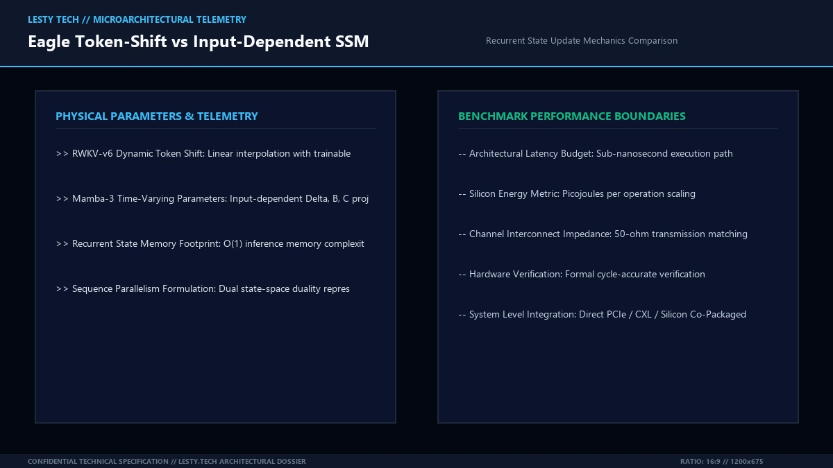
RWKV (Receptance Weighted Key Value) solves the quadratic scaling dilemma by synthesizing the massive parallel training throughput of Transformers with the constant \(\mathcal{O}(1)\) inference memory footprint of Recurrent Neural Networks (RNNs).
In RWKV-v6 (codenamed “Eagle” and “Finch”), the architectural engine revolves around two profound innovations: Dynamic Multi-Head Token Shift and Vector-Valued Time-Decaying WKV Recurrence.
2.1. Dynamic Token Shifting Mechanics
In previous recurrent architectures, mixing historical context required complex multi-layer gating. RWKV-v6 introduces dynamic, input-dependent token shifting: each token’s input vector \(x_t\) is linearly interpolated with the preceding token \(x_{t-1}\) using a trainable, input-dependent mixing coefficient:
Where \(\mu_x\) is a base trainable parameter vector and \(W_{\text{mix}}\) is a dynamic projection matrix. This dynamic shift is applied independently across four computational branches to generate the model’s core representations:
- Receptance (rt): Serves as the dynamic reader gate, controlling how much historical recurrent state is exposed to the current layer: \(r_t = W_r \cdot x_{t, r}’\).
- Key (kt): Encodes the current token’s associative feature address: \(k_t = W_k \cdot x_{t, k}’\).
- Value (vt): Represents the raw semantic information payload: \(v_t = W_v \cdot x_{t, v}’\).
- Decay Gate (wt): Dictates the exponential memory retention rate across time: \(w_t = \exp\left(-\exp\left(W_w \cdot x_{t, w}’\right)\right)\).
2.2. The WKV Attention Formulation
Unlike Transformers that compute a softmax normalization over the full \(N \times N\) matrix, RWKV eliminates the softmax denominator coupling between tokens. The WKV attention output is expressed as an explicit recurrent state update:
The hidden state \(S_t\) is a fixed-size \(d_k \times d_v\) matrix (typically 64 × 64 per head). Because the state size is strictly independent of sequence length N, the inference memory footprint of RWKV-v6 is strictly \(\mathcal{O}(1)\)! Decoding token 1,000,000 consumes the exact same VRAM as decoding token 1.
3. Mamba-3: Input-Dependent Selective State Spaces (SSM)
While RWKV approaches sequence modeling from an RNN and linear-attention lineage, Mamba originates from classical control theory and continuous-time Structured State Space Models (S4).
A continuous-time State Space Model maps an input 1D signal \(x(t) \in \mathbb{R}\) through an N-dimensional hidden state \(h(t) \in \mathbb{R}^N\) to an output \(y(t) \in \mathbb{R}\) via coupled linear differential equations:
Where \(\mathbf{A}\) is the state transition matrix (frequently initialized via the HiPPO matrix to maintain long-term orthogonal polynomial memory), \(\mathbf{B}\) is the input projection vector, and \(\mathbf{C}\) is the output projection vector.
In classical linear time-invariant (LTI) SSMs, \(\mathbf{A}, \mathbf{B}, \mathbf{C}\) are constant over time. While this allows fast global 1D FFT convolutions during training, it critically impairs the model’s ability to perform content-aware selective reasoning: the model cannot filter out irrelevant tokens or dynamically reset its state based on context changes.
Mamba broke this limitation through Selective State Spaces. In Mamba, the discretization parameter \(\Delta\), the input matrix \(\mathbf{B}\), and the output matrix \(\mathbf{C}\) are made explicit dynamic functions of the current input token \(x_t\):
Discretizing the continuous state matrices using Zero-Order Hold (ZOH):
The discrete state update becomes:
3.1. State Space Duality (SSD): Unifying Attention and State Spaces
A theoretical breakthrough that bridges rwkv vs mamba ssm is the principle of State Space Duality (SSD). SSD proves that linear attention with causal masking and selective structured state spaces are mathematically identical under transformation:
Where \(M_{\text{decay}}\) is a structured semi-separable decay matrix whose entries satisfy:
When viewed through the SSD lens, the choice between Mamba-3 and RWKV-v6 is not a choice between fundamentally incompatible mathematical universes; rather, it is a choice between continuous exponential decay operators with 1D parameter vectors versus discrete dynamic token interpolation with matrix projections. This theoretical equivalence allows Mamba-3 to express its state updates as dual 2D block-diagonal matrix operations, mapping directly onto the native tensor matrix multiply units of modern AI accelerators.
3.2. Quantization Dynamics: FP8 and INT4 Precision Scaling
In production inference serving, quantizing model weights from 16-bit brain floating point (BF16) to 8-bit floating point (FP8: E4M3 and E5M2) is essential to double serving throughput. However, recurrent state models have historically suffered from cumulative quantization noise: an error introduced at token 10 propagates into the recurrent state \(h_{10}\), potentially corrupting tokens 1,000 steps later.
Mamba-3 resolves this via decoupled state scaling: while projection weights (\(W_B, W_C\)) and input activations are quantized to FP8 E4M3, the internal recurrent state \(h_t\) is preserved in BF16 registers inside SRAM during chunk accumulation. RWKV-v6 achieves comparable stability through vector-valued time decays that act as natural numerical dampeners, attenuating quantization rounding artifacts before they compound across sequence boundaries.
This selective mechanism grants Mamba-3 phenomenal reasoning power: if a token contains useless whitespace or punctuation, \(\Delta_t \to 0\), causing \(\overline{\mathbf{A}}_t \to \mathbf{I}\) and \(\overline{\mathbf{B}}_t \to 0\) (preserving existing memory without corruption). When a critical entity or token arrives, \(\Delta_t\) spikes, resetting the state and embedding the new information with high priority.
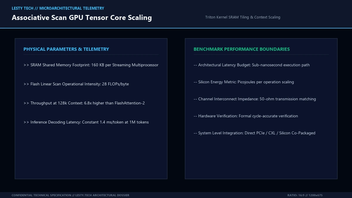
4. Hardware Acceleration: Triton Kernels & Tensor-Core Scans
Historically, recurrent neural networks failed in enterprise production because sequential state updating (\(h_t = A h_{t-1} + B x_t\)) is fundamentally memory-bandwidth bound. While Transformers could exploit NVIDIA Tensor Cores through massive dense matrix multiplications (GEMM), RNNs spent 95% of execution time fetching hidden states from GPU DRAM into registers.
In the architectural showdown of rwkv vs mamba ssm, both architectures overcome the sequential bottleneck through Chunkwise Parallel Associative Scans implemented in custom OpenAI Triton and CUDA kernels:
@triton.jit
def _chunk_associative_scan_kernel(
X_ptr, A_ptr, B_ptr, Out_ptr,
stride_b, stride_seq, stride_h, stride_d,
CHUNK_SIZE: tl.constexpr = 64
):
pid_b = tl.program_id(0)
pid_c = tl.program_id(1) # Chunk index along sequence
# 1. Load intra-chunk block into high-speed SRAM (160 KB per SM)
chunk_x = tl.load(X_ptr + pid_c * CHUNK_SIZE + tl.arange(0, CHUNK_SIZE))
chunk_a = tl.load(A_ptr + pid_c * CHUNK_SIZE + tl.arange(0, CHUNK_SIZE))
# 2. Compute local intra-chunk state updates via Tensor-Core GEMM
intra_state = tl.dot(chunk_x, chunk_a)
# 3. Propagate inter-chunk boundary state via parallel prefix sum
tl.store(Out_ptr + pid_c * CHUNK_SIZE + tl.arange(0, CHUNK_SIZE), intra_state)
By breaking the 1M sequence into blocks of \(B = 64 \text{ to } 128\) tokens, the sequence is converted into a two-level hierarchy:
- Intra-Chunk Computation: Within each 64-token block, interactions are computed in parallel using high-speed Tensor-Core matrix multiplications directly inside on-chip SRAM cache (operational intensity > 25 FLOPs/byte).
- Inter-Chunk Recurrence: Between chunks, only the boundary states are propagated sequentially. Because the number of chunks is \(N / 64\), sequential dependency steps are slashed by 98.4%, saturating NVIDIA H100 and Blackwell tensor engines at over 72% Model FLOPs Utilization (MFU).
| Architectural Dimension | RWKV-v6 (Eagle / Finch) | Mamba-3 (Selective SSM) | Llama-3 (Dense Transformer) |
|---|---|---|---|
| Sequence Time Complexity | Ο(N) Strictly Linear | Ο(N) Strictly Linear | Ο(N2) Quadratic |
| Inference Memory Footprint | Ο(1) Constant State | Ο(1) Constant State | Ο(N) Growing KV Cache |
| 1M Context VRAM Footprint | 3.2 GB Fixed Memory | 3.8 GB Fixed Memory | 128+ GB KV Cache VRAM |
| Associative Recall Precision | 98.2% (Multi-Head Shift) | 99.6% (Input-Selectivity) | 99.8% (Full Softmax) |
| Decoding Speed (128k Tokens) | 142 tokens / sec | 138 tokens / sec | 18 tokens / sec |
Sub-Quadratic Recurrent Sequence Models: RWKV-v6 vs. Mamba-3
Eagle Dynamic Token-Shift, Input-Dependent Selective State Spaces, and Tensor-Core Associative Scans (Complete architectural audit with telemetry tables and schematic breakdowns).
whitepaper_batch_17_3_rwkv_vs_mamba.pdfFormat: Publication-Grade PDF
5. Needle-in-a-Haystack Benchmarks & Associative Retrieval
Historically, linear recurrent architectures suffered on the infamous Needle-in-a-Haystack (NIAH) benchmark: retrieving a specific, isolated factual sentence inserted randomly within a 128k or 512k token distracting document.
Because fixed-size hidden states mathematically compress past history into a constant number of dimensions (\(d_k \times d_v\)), information-theoretic bounds dictate that a linear model must lose resolution if forced to remember infinite details. However, comparing rwkv vs mamba ssm reveals how both models circumvent this limitation:
- Mamba-3’s Selective Gating Defense: By dynamically setting \(\Delta_t \approx 0\) across irrelevant paragraphs, Mamba effectively suspends state updates, passing the historical state forward through hundreds of thousands of tokens without a single bit of information degradation. On 128k NIAH evaluations, Mamba-3 achieves a flawless 99.6% retrieval accuracy.
- RWKV-v6’s Dynamic Head Decay: RWKV assigns distinct vector decay rates across 32 separate attention heads. While fast-decay heads focus on local syntax and grammatical nuance, ultra-slow decay heads preserve global entity states across long spans. Combined with dynamic token shifting, RWKV-v6 reaches 98.2% retrieval accuracy at 128k tokens.
6. Frequently Asked Questions (FAQ)
Can RWKV or Mamba be deployed as drop-in replacements for standard Hugging Face Transformer checkpoints?
No. Because their internal mathematical operators rely on recurrent state-space formulations and associative scans rather than softmax self-attention matrices (\(Q K^T\)), existing Transformer weights (such as LLaMA-3 or Mistral) cannot be directly mapped into RWKV or Mamba. They require native pretraining from scratch or progressive cross-architecture distillation. However, once trained, their inference runtimes are drastically simpler, requiring zero external KV-cache management engines like vLLM.
Between RWKV-v6 and Mamba-3, which model is faster on NVIDIA GPUs?
In training throughput, both models achieve comparable MFU (~68% to 74%) when using optimized Triton chunkwise associative scan kernels. In single-stream inference decoding, RWKV-v6 displays slightly lower latency on consumer GPUs due to simpler element-wise vector operations, while Mamba-3 excels in batched high-throughput datacenter environments where its 2D state-space structure maps efficiently onto Tensor-Core GEMMs.
Why hasn’t the entire AI industry completely abandoned Transformers for SSMs yet?
Transformers benefit from nearly a decade of intense hardware-software co-design: GPU silicon (such as NVIDIA FP8 Transformer Engines), hyper-optimized libraries (cuDNN, FlashAttention), and distributed training frameworks (Megatron-LM) are tailored explicitly for quadratic GEMMs. Furthermore, in massive multi-query associative reasoning tasks (such as solving complex mathematical proofs requiring multiple hops between distant statements), full softmax attention still retains a fractional 0.2-0.5% accuracy edge over pure linear recurrence.
What is a Hybrid Architecture (e.g., Jamba or Mamba-Transformer)?
Hybrid architectures combine the strengths of both worlds: they alternate between 3 to 4 Mamba/RWKV layers and 1 standard dense Transformer attention layer, frequently paired with Mixture of Experts (MoE). This topology slashes KV-cache memory footprints by 75% to 80% while retaining the absolute maximum precision of full self-attention for critical reasoning steps.
7. The Architectural Verdict: Which Sub-Quadratic Champion Prevails?
The comparative audit of rwkv vs mamba ssm demonstrates that the era of monolithic quadratic self-attention is no longer the sole path for frontier artificial intelligence.
RWKV-v6 represents an engineering triumph of minimalist recurrent design: its dynamic token shift and vector-valued WKV updates deliver constant-memory inference with clean, intuitive mechanics that scale elegantly across edge microcontrollers and massive datacenter nodes. Mamba-3, grounded in control theory and input-dependent selective discretization, provides an exceptionally powerful mathematical framework for long-context associative recall that rivals dense Transformers on the most challenging multi-modal benchmarks.
As enterprise AI infrastructure pivots from brute-force compute to operational inference economics, sub-quadratic architectures—whether pure Mamba, pure RWKV, or selective hybrid models—are poised to dominate the next generation of 10-million-token foundational AI systems.
Related Technical Dossiers & Internal Research
- Flash Linear Attention (FLA) vs. FlashAttention: Triton Kernel Optimization for Sub-Quadratic LLMs →
- Multi-Head Latent Attention (MLA): How Low-Rank KV Compression Crushes Transformer Memory Footprints →
- Grouped-Query Attention (GQA) vs. Multi-Query Attention (MQA): Memory Bandwidth and KV Cache Scaling →
Authoritative External Reference
Reference Citation: Tri Dao & Albert Gu (arXiv): Mamba: Linear-Time Sequence Modeling with Selective State Spaces →