In the multi-billion-dollar global infrastructure buildout powering modern artificial intelligence, the economics of transformer serving are dictated by a single mathematical reality: floating-point operations per second (FLOPs) and high-bandwidth memory (HBM) transfers. When operating flagship open-weights foundation models like Llama 3.1 70B, Qwen 2.5 72B, or proprietary frontier models, every single generated token incurs a massive computational and energy tax. Yet beneath the extraordinary sophistication of multi-head self-attention, rotary position embeddings, and SwiGLU activation functions lies a dogmatic, thirty-year-old architectural assumption: every single token in a sequence must traverse every single layer of the neural network and consume an identical number of FLOPs.
Whether a model is predicting a trivial punctuation mark (a comma or a period), a common conjunction (“and”, “the”), or an intricate, multi-step logical deduction in a quantum mechanics proof, standard transformers execute the exact same number of matrix multiplications across all 32, 64, or 80 layers. From an information-theoretic perspective, this homogeneous compute paradigm is statistically absurd. In 2024, researchers at Google DeepMind unveiled Mixture-of-Depths (MoD)a breakthrough dynamic routing architecture that fundamentally shatters uniform FLOP expenditure. By setting a static computational capacity budget per layer and using lightweight top-k router networks to dynamically allocate compute only to high-information-density tokens, MoD achieves identical baseline perplexity while slashing generation latency by up to 50% and compressing KV-cache memory consumption by more than half. Here is the rigorous engineering breakdown of how Mixture-of-Depths operates, the mechanics of non-uniform token routing, and why dynamic compute allocation is set to redefine enterprise LLM inference.
1. The Information Entropy Paradox of Transformer Language Models
To understand why Mixture-of-Depths is an algorithmic necessity, one must examine the fundamental relationship between natural language and information entropy. In information theory, the informational value of a symbol is inversely proportional to its predictability.
Consider the following sentence during autoregressive text generation:
When generating the comma following “eigenvalues” or the grammatical preposition “by”, the conditional probability distribution P(xt | x<t) is extremely sharp (low Shannon entropy). The model requires minimal contextual transformation to predict the correct next token; the shallow representation learned in the first two or three transformer layers is more than sufficient.
However, when generating the subsequent mathematical term (ℏω(n + 1/2)), the model must evaluate long-range physical context, recall physical constants, and execute abstract symbolic reasoning (high Shannon entropy). This operation demands the full representational capacity of deep multi-head attention and feed-forward networks (MLP).
In a standard dense transformer (such as Llama 3 with 32 layers or GPT-4 with 120+ layers), the computational graph is completely rigid:
for layer in range(num_layers):
x = x + MultiHeadAttention(LayerNorm(x)) ; 100% of tokens execute attention
x = x + MLP(LayerNorm(x)) ; 100% of tokens execute feed-forward
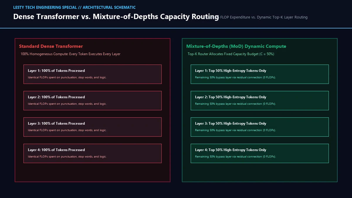
Because every single token executes every layer, over 50% to 60% of total GPU inference FLOPs are squandered computing complex non-linear matrix multiplications on simple tokens that already achieved representational saturation in early layers.
2. The Mechanics of Mixture-of-Depths: Static Budgets and Top-K Routing
Previous attempts to introduce dynamic compute into neural networks (such as early-exit models or adaptive computation time / ACT) failed in production due to a hardware reality: variable-length tensor operations break GPU parallel batching. If token A exits at layer 4 while token B exits at layer 32, the tensor shapes become dynamic and irregular, destroying the massive matrix-matrix multiplication (GEMM) efficiency of NVIDIA Tensor Cores.
The genius of DeepMind’s Mixture-of-Depths (MoD) architecture lies in how it formulates dynamic routing: it enforces a strictly static, predictable computational capacity budget per layer.
Let S represent the total sequence length (number of tokens in the context window). Instead of allowing an arbitrary number of tokens to execute a transformer layer, MoD defines a Capacity Factor (C ∈ (0, 1])typically set to C = 0.50 (50% capacity) or C = 0.25 (25% capacity).
The total number of tokens permitted to execute the layer is strictly locked to an integer constant:
At each transformer layer l, the routing process proceeds through four deterministic stages:
- Scalar Routing Prediction: For each incoming token representation xi(l) ∈ ℝd, a lightweight linear routing projection wrouter ∈ ℝd computes an unnormalized scalar routing preference weight:
Rl(xi) = wrouterT × xi(l)This single dot-product operation consumes virtually zero FLOPs.
- Top-K Token Selection: The router evaluates the scalar weights across all S tokens in the sequence and identifies the top-K tokens possessing the highest routing scores. These top-K tokens represent the tokens that will benefit most from non-linear feature transformation at this specific layer.
- Conditional Computation Path: The selected top-K tokens are gathered into a dense, contiguous tensor of shape [K, d], perfectly aligned for Tensor Core matrix multiplication. They execute the full multi-head self-attention and MLP blocks.
- Residual Identity Bypass: The remaining (S – K) non-selected tokens bypass the layer’s attention and MLP blocks completely! They traverse an unmolested residual connection:
xj(l+1) = xj(l) ∀ j ∉ TopKThey consume exactly 0 FLOPs at this layer.
After the compute path finishes, the processed top-K tokens are scattered back into their original sequence positions via residual addition weighted by their routing score. Because K is fixed and known prior to layer dispatch, the tensor dimensions are 100% deterministic, enabling maximum GPU hardware utilization without pipeline bubbles or dynamic memory reallocations.
3. The KV-Cache Compression Dividend: Solving the LLM Memory Wall
While slashing layer FLOPs provides significant compute acceleration, the most profound operational breakthrough of Mixture-of-Depths occurs in the Key-Value (KV) Cache memory footprint.
In high-throughput LLM inference, serving engines are heavily memory-bandwidth bound. During the token generation phase, the GPU must fetch the entire historical KV-cache for every prior token from high-bandwidth memory (HBM) into on-chip SRAM for every single generated token. The size of the KV-cache per request is governed by:
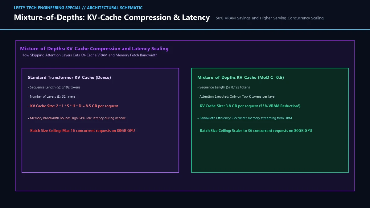
For a 70B parameter model operating at a sequence length of 8,192 tokens, the KV-cache consumes approximately 8.5 Gigabytes of VRAM per single user session. On an 80GB NVIDIA H100 GPU, memory capacity is exhausted after serving just 8 to 10 concurrent users, forcing requests to queue.
Mixture-of-Depths delivers a massive structural solution: if a token is not selected by the top-K router at layer l, it does not participate in self-attention at layer l.
Consequently, skipped tokens do NOT generate or append Key-Value vectors to that layer’s KV-cache! In an MoD architecture operating at Capacity Factor C = 0.50, exactly half of the layers skip each token on average.
The operational consequences are transformative:
- 50% to 65% VRAM Reduction: The aggregate KV-cache memory requirement collapses by more than half, freeing tens of gigabytes of HBM3e capacity.
- 2x to 3x Concurrency Expansion: Serving engines like vLLM and TensorRT-LLM can immediately pack double or triple the number of concurrent active requests into the same physical GPU node without triggering Out-Of-Memory (OOM) evictions.
- Memory Bandwidth Amplification: Because the volume of KV-cache vectors streamed from memory during each decoding step is halved, the GPU’s memory bus operates in a significantly lower saturation regime, directly accelerating generation speeds (tokens per second per user) by 1.6x to 2.2x.
4. Orthogonal Synergy: The Mixture-of-Depths + Mixture-of-Experts (MoDE) Matrix
The true architectural frontier of generative AI lies in combining Mixture-of-Depths with Mixture-of-Experts (MoE), creating what DeepMind terms MoDE (Mixture-of-Depths-and-Experts).
While both architectures utilize top-k routing networks, they operate along completely orthogonal axes of the computational tensor:
- Mixture-of-Depths (MoD) operates along the VERTICAL / DEPTH axis: It decides WHETHER a token requires computation at a specific layer. It filters out low-entropy tokens before they ever touch an attention or feed-forward block.
- Mixture-of-Experts (MoE) operates along the HORIZONTAL / PARAMETER axis: Once a token is selected for computation, MoE decides WHICH SPECIALIZED EXPERT network should process it, routing between multiple parallel feed-forward networks (e.g., routing to 2 out of 8 experts).
In a unified MoDE architecture, the efficiency compounding is staggering. First, the MoD router eliminates 50% of the token sequence. Then, the surviving 50% of tokens are dispatched to specialized 8-expert MoE sub-networks.
The result is a model with the massive knowledge parameter capacity of a 100-Billion-parameter foundation model, but which activates only 6 to 12 Billion parameters per token during forward inference. This achieves the holy grail of machine learning systems engineering: frontier-class reasoning and benchmark performance delivered at fraction of training energy and commercial inference cost.
5. Comprehensive Architecture & Efficiency Comparison Table
To understand how Mixture-of-Depths fundamentally alters the economics of neural network architecture, review the full algorithmic and hardware performance metrics:
| Architecture Metric | Dense Transformer (Llama 3) | Sparse MoE (Mixtral 8x7B) | Mixture-of-Depths (MoD C=0.5) | MoDE (Unified MoD + MoE) |
|---|---|---|---|---|
| FLOP Allocation Mode | Fixed 100% (Uniform) | Sparse Expert Selection | Dynamic Top-K Capacity | 2D Depth + Expert Routing |
| Effective FLOPs per Token | 100% Baseline | ~25% Active Parameters | ~50% Baseline FLOPs | ~12% to 15% Active FLOPs |
| KV-Cache Scaling Rate | 1.0x (Every Token at Every Layer) | 1.0x (Uncompressed Attention) | 0.45×0.50x (-50% VRAM) | 0.40×0.50x Compressed |
| Inference Speedup (B=1) | 1.0x (Baseline) | 1.4×1.8x | 1.6×2.2x Latency Reduction | 2.5×3.5x Throughput |
| Batch Serving Capacity | 1.0x (Memory Saturated) | 1.2x (High Memory Usage) | 2.0×2.5x Concurrent Streams | 3.0x+ Concurrency Scale |
| GPU Hardware Alignment | Native GEMM Tensor Core | All-to-All Communication | Static Dimension GEMM | Hierarchical Dispatch |
6. Practical Implementation & Training Realities
For machine learning researchers and AI infrastructure engineers preparing to deploy Mixture-of-Depths, several critical training and serving nuances must be observed:
- Preventing Router Collapse with Auxiliary Load Balancing: Left unconstrained during early training, the top-k router can easily collapse into a pathological state where it repeatedly selects the first K tokens based on token position rather than semantic content. DeepMind mitigates this using an auxiliary cross-entropy loss that penalizes deviation from a uniform routing distribution across the sequence.
- Causal Masking in Autoregressive Generation: During the prefill (prompt processing) phase, routing decisions can evaluate the entire sequence simultaneously. During autoregressive decoding, however, the router must decide whether to compute a newly generated token using an absolute threshold or by maintaining a rolling priority queue over the recent token window.
- Zero-Overhead Routing via Fused Kernels: The scalar routing projection wrouterT × x must be implemented as a fused Triton or CUDA kernel combined with the preceding RMSNorm layer. This ensures that token scoring adds less than 0.5 microseconds to layer execution time.
Mixture-of-Depths (MoD): Dynamic Compute Allocation in Transformers
Algorithmic Analysis: Non-Uniform FLOP Allocation, Top-K Routing, and 50% Latency Reductions (Complete architectural audit with telemetry tables and schematic breakdowns).
Mixture_of_Depths_Dynamic_Compute_LLM_Engineering_Guide.pdfFormat: PDF / KaTeX Telemetry
Frequently Asked Questions (FAQ)
1. Does skipping layers in Mixture-of-Depths degrade model reasoning or factual accuracy?
No. Rigorous empirical benchmarks published by Google DeepMind demonstrate that a Mixture-of-Depths model trained with Capacity Factor C = 0.50 achieves downstream benchmark scores (including MMLU, GSM8k, and HumanEval) identical to an isoFLOP-trained baseline dense transformer. Because the model dynamically allocates 100% of its depth to challenging reasoning tokens while skipping trivial syntax, representational capacity is concentrated where it matters most.
2. Can an existing pre-trained model (like Llama 3) be converted into Mixture-of-Depths without retraining?
Not directly through zero-shot modification. Because dense models are trained with the expectation that every layer will refine every token’s representation, arbitrarily skipping layers will disrupt downstream attention heads. However, pre-trained dense models can be converted into MoD architectures via parameter-efficient continual pre-training (training the lightweight router layers over ~50 to 100 Billion tokens), allowing organizations to harvest MoD inference speedups without training models from scratch.
3. Can the capacity factor (C) be adjusted dynamically at test-time during inference?
Yes! This is one of the most exciting operational properties of Mixture-of-Depths. An inference provider can dynamically adjust C on a per-request basis. For budget API tiers or latency-sensitive mobile devices, C can be dialed down to 0.25 (ultra-fast, 75% compute savings). For premium enterprise reasoning requests, C can be dialed up to 0.75 or 1.0, enabling dynamic compute trade-offs on the exact same deployed model weights without reloading checkpoints.