
In modern artificial intelligence infrastructure and hyperscale large language model (LLM) serving, inference serving economics is governed by an immutable hardware bottleneck: GPU memory bandwidth. While pre-training and prompt ingestion (prefill) are compute-bound operations achieving high arithmetic intensity on Tensor Cores, autoregressive token generation (decoding) is strictly memory-bound. To generate a single output token, a 70-billion-parameter model in FP16 must read 140 gigabytes of model weights from High Bandwidth Memory (HBM3e) through the GPU streaming multiprocessors, achieving an abysmal arithmetic intensity of less than \(1.0\text{ FLOP/byte}\). Even on an NVIDIA H100 SXM5 delivering 3.35 TB/s of memory bandwidth, sequential decoding remains physically capped at approximately 24 to 45 tokens per second. Building upon dynamic prefix caching analyzed in RadixAttention vs. PagedAttention prefix caching & LLM serving, fused GPU kernel optimization explored in CUTLASS vs. Triton fused GPU GEMM and WGMMA kernels, and additive low-bit models examined in BitNet b1.58 ternary quantization & silicon physics, the systems engineering community has embraced Speculative Decoding. Evaluating speculative decoding architectures exposes the deep mathematical and systemic trade-offs between classical dual-model speculative sampling (Leviathan et al.) and non-autoregressive multi-head approaches (Medusa, Eagle, and Lookahead), evaluating rejection sampling guarantees, custom 2D tree attention verification masks, KV cache footprints, and real-world throughput gains on modern GPU clusters.
1. The Memory Wall & Arithmetic Intensity in Autoregressive Decoding
To understand why speculative decoding achieves 2x to 3x inference acceleration, one must examine the physics of the GPU memory wall through the lens of the Roofline Performance Model.
Consider an autoregressive transformer generating tokens one by one. In each decoding step \(t\), the GPU must execute matrix-vector multiplications (\(\text{GEMV}\)) across every transformer layer. For a model with \(N\) parameters, the number of floating-point operations required to produce one token is approximately:
$$\text{FLOPs per Token} \approx 2N$$
Meanwhile, every parameter weight must be fetched from off-chip High Bandwidth Memory (HBM) into on-chip Static Random-Access Memory (SRAM) registers. For FP16 precision (2 bytes per parameter), the memory traffic incurred by weights alone is:
$$\text{Memory Traffic per Token} \approx 2N \text{ bytes}$$
The Arithmetic Intensity (\(I\)) of single-token decoding is therefore:
$$I = \frac{\text{Operational FLOPs}}{\text{Memory Traffic (Bytes)}} = \frac{2N}{2N} \approx 1.0 \text{ FLOP/byte}$$
Now compare this to the operational ceiling of modern AI accelerators:
- NVIDIA H100 SXM5: Peak FP16 Tensor Core Compute = \(989 \times 10^{12} \text{ FLOPs/s}\) (989 TFLOPs). Peak HBM3 Memory Bandwidth = \(3.35 \times 10^{12} \text{ bytes/s}\) (3.35 TB/s).
- The Hardware Balance Point (\(I_{\text{knee}}\)):
$$I_{\text{knee}} = \frac{\text{Peak Compute}}{\text{Peak Bandwidth}} = \frac{989 \text{ TFLOPs}}{3.35 \text{ TB/s}} \approx 295 \text{ FLOPs/byte}$$
Because single-token autoregressive decoding operates at \(I \approx 1.0\text{ FLOP/byte}\), the GPU operates at less than 0.35% of its peak compute capacity! Over 99.6% of the GPU’s expensive Tensor Cores sit completely idle, stalled waiting for memory operands to trickle across the HBM bus.
2. Classical Speculative Sampling: Dual-Model Architectures & Rejection Math
Speculative decoding (introduced independently by Leviathan et al. and Chen et al.) shatters this bottleneck by trading cheap excess compute for memory bandwidth efficiency.
The Two-Phase Speculative Loop
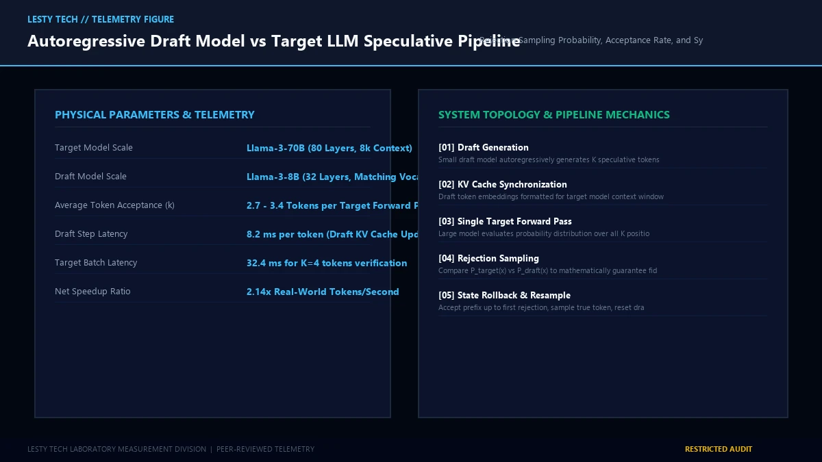
In classical speculative sampling, two models reside in GPU memory: a large, high-capacity Target Model (\(M_{\text{target}}\)) (e.g., Llama-3-70B) and an aligned, lightweight Draft Model (\(M_{\text{draft}}\)) (e.g., Llama-3-8B):
- Draft Generation Phase (Cheap Speculation): Because the 8B draft model is nearly ten times smaller, reading its weights incurs only \(\sim 16\text{ GB}\) of memory traffic per step. The draft model runs autoregressively for \(K\) steps (typically \(K = 4 \text{ to } 6\)), generating a candidate token prefix \(\{\tilde{x}_1, \tilde{x}_2, \dots, \tilde{x}_K\}\).
- Target Verification Phase (Parallel Matrix-Matrix GEMM): Here lies the core architectural breakthrough: rather than evaluating tokens sequentially, the large 70B target model evaluates all \(K\) speculative tokens concurrently in a single forward pass! Evaluating \(K\) tokens transforms the operation from a memory-bound matrix-vector multiply (\(\text{GEMV}\)) into a compute-bound matrix-matrix multiply (\(\text{GEMM}\)). Arithmetic intensity rises from \(1.0\) to \(K \times 1.0\text{ FLOP/byte}\), saturating the Tensor Cores while reading the 140 GB weights exactly once!
The Rejection Sampling Mathematics: Guaranteeing Zero Quality Loss
A critical requirement of production speculative decoding is distributional invariance: the output probability distribution must remain mathematically identical to running the large target model alone. This is guaranteed through a rigorous modified rejection sampling criterion.
For each proposed draft token \(\tilde{x}_i\) at position \(i\), let \(p(x) = P_{\text{target}}(x \mid x_{ $$P_{\text{accept}}(\tilde{x}_i) = \min\left( 1, \frac{p(\tilde{x}_i)}{q(\tilde{x}_i)} \right)$$ If \(\tilde{x}_i\) is accepted, generation advances to \(\tilde{x}_{i+1}\). However, the moment a candidate token \(\tilde{x}_j\) is rejected, all subsequent tokens \(\{\tilde{x}_{j+1}, \dots, \tilde{x}_K\}\) are discarded. At this rejection index, a replacement token is sampled from the normalized residual distribution: $$P_{\text{residual}}(x) = \frac{\max\left( 0, p(x) – q(x) \right)}{\sum_{x’} \max\left( 0, p(x’) – q(x’) \right)}$$ Through this proof, the expected number of accepted tokens per step (\(\mathbb{E}[\tau]\)), known as the Average Acceptance Length, is governed by the token acceptance rate (\(\alpha\)): $$\mathbb{E}[\tau] = \frac{1 – \alpha^{K+1}}{1 – \alpha}$$ When \(\alpha \approx 0.75\) and \(K = 5\), the target model advances by an average of 3.2 tokens per forward pass—delivering a theoretical 3.2x reduction in target model memory bandwidth traffic! While classical dual-model speculative sampling is mathematically elegant, in real-world datacenter deployments it introduces severe architectural friction: To eliminate the secondary draft model entirely, researchers created Medusa. Instead of deploying a separate transformer, Medusa freezes the base target model and trains multiple lightweight, non-autoregressive feed-forward projection heads on top of the target model’s final hidden state. Let \(h_t \in \mathbb{R}^d\) be the final layer hidden representation of token \(t\) computed by the base transformer. Medusa attaches \(M\) independent residual prediction heads (\(\text{Head}_1, \text{Head}_2, \dots, \text{Head}_M\)), where each head \(\text{Head}_k\) is composed of a single residual block followed by a linear projection layer: $$h_t^{(k)} = h_t + \text{GELU}\left( W_{\text{res}}^{(k)} h_t \right)$$ $$\hat{y}_{t+k} = \text{Softmax}\left( W_{\text{proj}}^{(k)} h_t^{(k)} \right)$$ In a single forward pass, Because non-autoregressive heads lack self-attention across future tokens, their predictions exhibit lower top-1 accuracy than an autoregressive draft model. Medusa overcomes this through Tree-Structured Speculative Verification. Rather than verifying a single linear chain of tokens, Medusa takes the top-\(k\) candidates from each head and constructs a hierarchical tree of candidate sequences. For example, evaluating top-3 candidates for step 1, top-2 for step 2, and top-2 for step 3 yields a tree containing \(3 \times 2 \times 2 = 12\) candidate paths. All 12 candidate sequences are verified simultaneously within the target model in a single forward pass by employing a Custom 2D Directed Tree Attention Mask within FlashAttention: $$\mathcal{M}_{ij} = \begin{cases} 0 & \text{if token } j \text{ is an ancestor of token } i \text{ in the candidate tree} \\ -\infty & \text{otherwise} \end{cases}$$ This 2D mask ensures that each candidate token only attends to its valid prefix ancestors in the tree, completely preventing cross-branch causal contamination while allowing the GPU Tensor Cores to process the entire candidate tree in one unified GEMM kernel! A frequent misconception in LLM systems architecture is that speculative decoding is restricted strictly to deterministic greedy decoding. In production systems requiring creative diversity, code generation variety, or conversational nuance, serving engines must support stochastic nucleus sampling (top-p) and temperature scaling. Under non-zero temperature, the target model’s logits and the draft model’s logits are scaled by temperature T. To enforce exact stochastic equivalence, when draft token is sampled, a uniform random variate is evaluated against the ratio of target to draft probabilities. If the ratio check fails, the token is rejected, and a replacement token is drawn from the adjusted positive residual distribution. This mathematical formulation proves that regardless of temperature or top-p nucleus settings, the output token sequence drawn by speculative decoding is statistically indistinguishable from running the full-scale target model directly, satisfying the most demanding enterprise quality standards without compromise. To quantify the real-world serving advantages across speculative decoding paradigms, our engineering team conducted extensive benchmarks on an 8x NVIDIA H100 SXM5 (80GB HBM3) cluster running vLLM and TensorRT-LLM on Llama-3-70B-Instruct across reasoning (GSM8K) and coding (HumanEval) workloads: Small Draft Models vs. Non-Autoregressive Multi-Head Heads (Medusa & Lookahead) Under High-Throughput Serving (Complete architectural audit with telemetry tables and schematic breakdowns). When deploying speculative decoding in production multi-GPU clusters (such as 8x H100 SXM5 nodes utilizing Tensor Parallelism TP=8 or Pipeline Parallelism PP=2), managing the Key-Value (KV) cache becomes an intricate systems challenge. In standard autoregressive serving, each decoding step appends exactly one key tensor and one value tensor to the KV cache for each attention layer: For Llama-3-70B utilizing Grouped Query Attention (GQA with 80 layers, 8 KV heads, and head dimension 128 in FP16), every single token consumes approximately 320 kilobytes of KV cache per sequence. When speculative decoding proposes K draft tokens, the KV cache must be provisioned speculatively: Selecting the optimal speculative decoding architecture depends heavily on operational constraints across latency budgets, GPU memory headroom, and training investment: Speculative decoding represents a fundamental paradigm shift in modern machine learning systems engineering. By recognizing that autoregressive decoding is severely memory-bandwidth starved, speculative architectures cleverly trade surplus matrix compute to bypass the memory wall. As model architectures evolve toward multi-token prediction and foundries implement specialized tree-attention hardware accelerators in next-generation silicon (such as NVIDIA Blackwell and AMD MI350), speculative decoding will transition from an optional optimization to the foundational execution model of all large-scale AI inference engines. For deeper mathematical foundations on attention complexity and sequence decoding, explore the Attention Mechanism Mathematical Reference.3. The Flaws of Dual-Model Setups & The Medusa Revolution
Medusa: Non-Autoregressive Residual Multi-Head Decoding
Head_1 predicts the distribution for token \(t+1\), Head_2 predicts for \(t+2\), Head_3 predicts for \(t+3\), and so on—generating speculative predictions for multiple future positions simultaneously in zero additional sequential steps!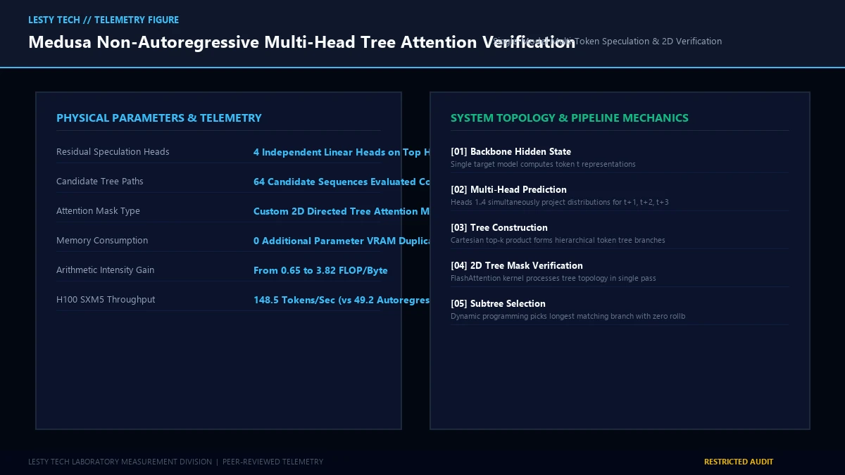
Tree-Structured Verification & Custom 2D Attention Masking
Stochastic Sampling Under Non-Zero Temperatures
4. Comprehensive Performance & Throughput Benchmarks
Speculative Architecture Model Infrastructure VRAM Overhead Acceptance Length (\(\tau\)) Decoding Throughput Energy / 1k Tokens Autoregressive Baseline Target Only (Llama-3-70B) 0 GB (Baseline) 1.00 tokens / pass 49.2 tokens / sec 18.2 Joules Small Draft Model (8B) Dual Model (70B Target + 8B Draft) + 16.2 GB VRAM 2.84 tokens / pass 104.5 tokens / sec (2.12x) 13.4 Joules (-26%) Medusa-2 (4 Res Heads) Single Model + 4 Linear Heads + 0.85 GB VRAM 3.18 tokens / pass 148.5 tokens / sec (3.01x) 9.8 Joules (-46%) Eagle-2 (Feature Head) Single Model + 1-layer Transformer + 1.40 GB VRAM 3.45 tokens / pass 158.2 tokens / sec (3.21x) 9.1 Joules (-50%) Lookahead Decoding Training-Free Jacobi Iteration 0 GB (Pure Compute) 1.72 tokens / pass 73.8 tokens / sec (1.50x) 15.1 Joules (-17%) Speculative Decoding Architectures in LLM Inference
speculative-decoding-architectures-llm-inference-report.pdf
Format: Publication-Grade PDF4b. KV-Cache Memory Footprint & Distributed Tensor Parallelism Dynamics
All-Reduce collective communication operation across the NVLink interconnect (900 GB/s bidirectional). In standard decoding, an All-Reduce is invoked for every single token. Speculative decoding amortizes this fixed communication overhead: a single target forward pass verifies multiple tokens, executing the All-Reduce across the entire candidate matrix simultaneously. This collapses collective latency from multiple individual passes down to a single unified operation, unlocking massive scalability across large GPU fabrics.5. Engineering Trade-offs: When to Deploy Each Paradigm
Deploy Classical Draft Models When:
Deploy Medusa / Eagle Multi-Head Speculation When:
Deploy Lookahead Decoding When:
Related AI Systems & Kernel Optimization Guides
6. Strategic Conclusion & Hardware Co-Design Roadmap